Cybersecurity is concerned with the privacy and security of computers or electronic devices, networks, and any information that is stored, processed, or exchanged by information systems [1]. Parameter design, monitoring, and network maintenance are important to network cybersecurity. The detection and prevention of attacks are generally more significant than any subsequent actions taken after being attacked [2]. It is helpful to obtain as much information as possible from attacks to defend against attackers and improve the cybersecurity of information systems [3]. A honeypot system can collect information from an attack about the attackers and may aid in the practice of robust cybersecurity. A honeypot is used to attract attackers and record their activities [4].

Attackers can be attracted to a fake system by a honeypot in the network infrastructure; valuable information can be obtained from them; and the information can then be used to improve network security [4]. A honeypot constitutes a useful technique or tool to observe the spread of malware and the emergence of new exploits. An attacker tries to avoid connecting to a honeypot as it can disclose the attacker’s tools, methods, and exploits [5]. A honeypot is also a source that can be leveraged to build high-quality intelligence against threats, providing a means for monitoring attacks and discovering zero-day exploits [6]. A network honeypot is often used by information security teams to measure the threat landscape for the security of their networks [7]. One example of a stochastic process method, the MDP, has been used for decision-making in cybersecurity. The MDP assumes that both defenders and attackers have observable information, although this is not true in many applications [8]. In actuality, there may be partial observability or an agent’s inability to fully observe the state of its environment in numerous real situations [9]. In many real-world problems, their environmental models are not known. There is a considerable need for reinforcement learning to solve problems where agents partially observe the states of their environments (possibly due to noise in the observed data). This leaves the outcomes of actions under uncertainty more dependent on the signal of the current state. The POMDP extends the MDP by permitting a decision-making process under uncertain or partial observability [10]. The artificial intelligence (AI) world has shown a huge leap recently in the research area of the POMDP model [11].

An MDP model for interaction honeypots was created and an analytic formula of the gain was derived. The optimal policy was decided based on comparing the calculated gain of each policy and selecting the one with a maximal gain. The model was then extended using a POMDP. One approach to solving the POMDP problem was proposed. In this method, the system state was replaced with the belief state and the POMDP problem was converted into an MDP problem [12]. The efforts in the research of this paper were to fulfil predictive modelling of the honeypot system, based on the MDP and the POMDP. Various methods and algorithms were used, including VI, PI, LP, and Q-learning in the analyses of the discounted MDP over an infinite planning horizon. The results of these algorithms were evaluated to validate the created MDP model and its parameters. In the modelling of the discounted POMDP over an infinite planning horizon, the effects of several important parameters on the system’s total expected reward were studied. These parameters include the observation probability of receiving commands, the probability of attacking the honeypot, the probability of the honeypot being disclosed, and the transition rewards. The analyses of the MDP and POMDP in this paper were conducted using the R language and R functions. This paper is organised as follows: the second section introduces the methods of MDP and POMDP; Section 3 presents a created MDP model of the system and the parameters in the model; Section 4 shows the analyses of the system based on the MDP method; Section 5 presents analyses of the system based on the POMDP method, and the final section is the conclusion.

2.1. The MDP

The MDP method is one of the most significant methods employed in artificial intelligence (especially machine learning). The MDP is described using the tuple <S, A, T, R, γ> [13–15]:

• S is the states’ set. • A is the actions set. • T is the transition probability from the state s to the state s′ (s ∈ S, s′ ∈ S) after action a (a ∈ A). • R is an immediate reward after action a, and • γ (0 < γ < 1) is the discounted factor.

An optimal policy is the goal of the MDP that maximises the total expected reward. An optimal policy over a finite planning horizon maximises the vector of the total expected reward until the horizon ends. The total expected reward (discounted) for an infinite planning horizon is employed to evaluate the gain of the discounted MDP in this paper.

2.2. The Algorithms of the MDP

VI, PI, LP, and Q-learning have been the algorithms utilised to find an optimal policy for the MDP. Theoretically, the results of the four kinds of algorithms should be the same. However, the results obtained using the algorithms may potentially differ with a great value, or convergence problems may potentially occur during the iterative process if the created MDP model is unreasonable, owing to unsuitable structure or incorrect model parameters. Thus, all the algorithms are employed, and their results are evaluated to validate the model constructed in this paper.

VI: An optimal policy for the MDP can be achieved by utilizing VI when the planning horizon is finite. In principle, the four algorithms (VI, PI, LP, and Q-learning) can be employed to find the optimal policy when the planning horizon is infinite. VI utilises the following equation of value iterations [16–18] to calculate the total expected reward for each state:

where T(s, a, s′ ) is the transition probability from state s to state s′ after action a. R(s, a, s′ ) is the immediate reward of the transition. V(s) and V(s′ ) are the total expected reward in state s and state s′ , respectively. When the value difference between 2 consecutive iterative steps is lower than the given tolerance, the iteration will be stopped.

PI: A better policy is found using PI, through comparing the current policy to the previous one. PI generally begins arbitrarily with an initial policy and then policy evaluation and policy improvement are followed. The process of iterations continues until the same policy is obtained for 2 successive policy iterations, indicating that the optimal policy has been achieved. For each state s, Equation (2) is used for policy evaluation and Equation (3) is used for updating the policy (policy improvement) [16, 18].

where π(s) is an optimal policy of state s.

LP: Since the MDP can be expressed as a linear program, the LP can find a static policy through solving the linear program. The following LP formulation [19] is used to find the optimal value function:

subject to

Q-learning: It is used to achieve the best policy with the greatest reward. It is a reinforcement learning method and allows an agent to learn the Q-value function that is an optimal action-value function. Q-learning can also be applied to non-MDP domains [20]. The action-value function Q(s, a) is expressed as follows [21]:

Q(s, a) can be initialised arbitrarily (for example, Q(s, a) = 0, ∀s ∈ S, ∀a ∈ A). From state s to state s′ , a Q-learning update can be defined as follows [21, 22]:

where β ∈ (0, 1) represents the learning rate. The best action a at state s can be chosen according to the optimal policy π(s). The iterative process continues until the final step of episode. The optimal policy is described as follows:

2.3. The POMDP

A POMDP can be thought as a generalisation of an MDP, permitting state uncertainty in a Markov process [23]. In POMDP applications, the objective is generally to obtain a decision rule or policy to maximise the expected long-term reward [24]. In the POMDP, the belief state is a distribution of probabilities over all possible states. An optimal action relies only on the current belief state [25].

The POMDP was defined as a tuple <S, A, T, R, O, B, γ> [26]:

• O = {o1, o2, ..., ok} is an observation set. • B is a set of conditional observation probabilities B(o|s′ , a). s′ is the new state after the state transition s → s′ , o ∈ O. • S, A, T, R, and γ are the same as those in the tuple of MDP.

After having taken the action a and observing o, the belief state needs to be updated. If b(s) is the previous belief state, then the new belief state [25] is given by

where a is a normalizing constant that makes the belief state sum to 1.

The goal of POMDP planning is to obtain a sequence of actions {a₀, a₁, ..., a_t} at time steps that maximise the total expected reward [27], i.e., we choose actions that give

where st and at are the state and the action at time t, respectively

The optimal policy brings up the greatest expected reward for each belief state, which is the solution to the Bellman optimality equation through iterations beginning at an initial value function for an initial belief state. The equation can be formulated as [12]:

3.1. The Structure of the MDP Model

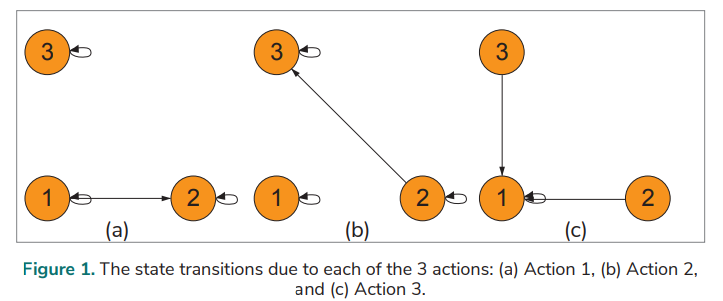
The honeypot system is a network-attached system that is put in place to lure attackers. A botnet is utilised to forward spam, steal data, etc. A botmaster keeps a bot online. A honeypot has three states [12]:

• State 1: Not attacked yet (waiting for an attack to join the botnet). • State 2: Compromised (becoming a member of the botnet). • State 3: Disclosed (not the botnet’s member anymore) due to the real identity having been discovered or interactions with the botmaster having been lost for an extended period of time.

A honeypot can take one of the following actions at each state:

• Action 1: Allows a botmaster to compromise the honeypot system and to implement commands. • Action 2: Does not allow the botmaster to compromise the system. • Action 3: Reinitialised as a new honeypot and reset to the initial state.

A model of the honeypot system is established based on the MDP. Fig. 1. shows the state transitions of the states (1, 2, and 3) resulted from each of the actions (Action 1, Action 2, and Action 3).

Figure 1. The state transitions due to each of the 3 actions: (a) Action 1, (b) Action 2, and (c) Action 3.

3.2. State Transition Matrix and Reward Matrix

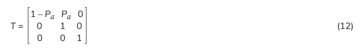
The transitions between the states in the created model of the system rely on one of the actions and on two important probabilities [12]. State 1 cannot be transitioned to State 3 directly; State 3 cannot be transitioned to State 2. The probability of a transition from State 3 to State 1 is 0 (under Action 1 or Action 2) or 1 (under Action 3). The following is a description of the two important probabilities:

• P_a : the probability of attacking the honeypot. • P_d : the probability of the honeypot being disclosed.

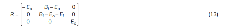
The benefit and expenses due to the state transitions or self-transitions are as follows [12]:

• E_o: the operation expense due to running, deploying, and controlling a honeypot. • E_r: the expense in reinitializing a honeypot. • E_l : the expense in liability when a honeypot operator becomes liable for implementing a botmaster’s commands if those commands include illicit actions. • B_i : the benefit of information when a honeypot collects an attacker’s information regarding techniques, codes, and tools.

The state transition probability matrix T and the reward matrix R under each action are formulated as follows:

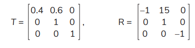
1) T and R under Action 1 are

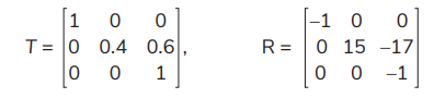
2) T and R under Action 2 are

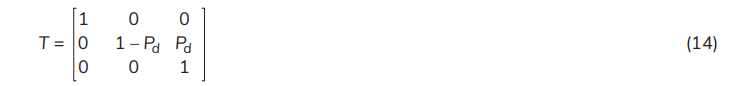
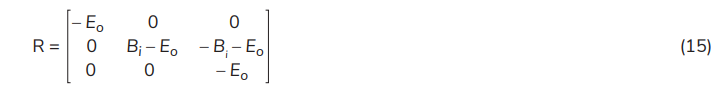
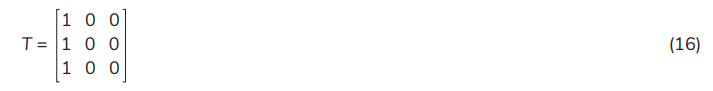
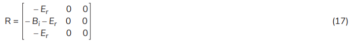
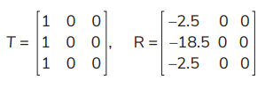
3) T and R under Action 3 are

4.1. MDP-based Analyses over an Infinite Planning Horizon

Let P_a = 0.6, P_d = 0.6, E_o = 1, E_r = 2.5, B_i = 16, E_l = 14, and γ = 0.85. Analyses are performed using the R language and its functions. By substituting the data into equations (12–17), the values of T and R under various actions (due to various policies) can be computed:

T and R under Action 1 become

T and R under Action 2 are

T and R under Action 3 are

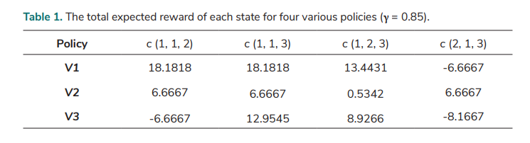
Various policies are evaluated, and Tab. 1. shows the result of the total expected rewards for states with various policies. For example, the policy c (1, 1, 3) indicates that Action 1, Action 1, and Action 3 are taken on State 1, State 2, and State 3, respectively. V1, V2, and V3 represent the total expected reward for State 1, State 2, and State 3, respectively.

Table 1. The total expected reward of each state for four various policies (γ = 0.85).

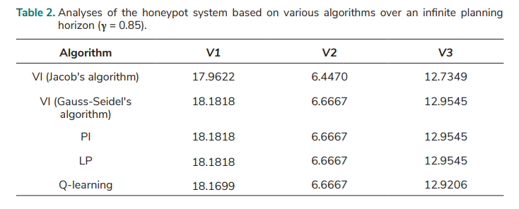
The four kinds of algorithms (VI, PI, LP, and Q-learning) can be implemented using the values of T and R under various actions. These algorithms are used in this paper and the optimal policy achieved using the four algorithms is c (1, 1, 3) in each case. The results for the total expected rewards for each state are compared to evaluate the validity of the MDP model in this paper. The results of the honeypot system (based on a discounted MDP with γ = 0.85) over an infinite planning horizon are shown in Tab. 2.

VI consists of solving Bellman’s equation iteratively. Jacob’s algorithm and Gauss-Seidel’s algorithm are employed in the VI method respectively, so that there are two variants of VI algorithm employed. In Gauss-Seidel’s value iterations, V(k+1) is used instead of V(k) whenever this value has been calculated; k is the iteration number. In this situation, the convergence speed is enhanced. It is also shown that its accuracy is improved in comparison to Jacob’s algorithm (Tab. 2.). The result of Gauss-Seidel’s value iteration algorithm shows that the total expected reward is 18.1818 (the highest value) if the MDP starts in state 1 while it is 6.6667 (the lowest value) if the MDP starts in state 2. The Q-learning result in Tab. 2. was obtained when the number of iterations was 150,000. The results of the VI (Gauss-Seidel's algorithm), PI, and LP are the same, and very close to the Q-learning result, indicating the MDP model created is valid, and that the model parameters are indeed suitable.

Table 2. Analyses of the honeypot system based on various algorithms over an infinite planning horizon (γ = 0.85).

4.2. The MDP-based Analysis for the Honeypot System over a Finite Planning Horizon

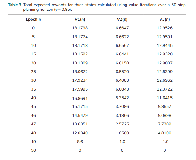
The above data regarding probabilities, the benefit, and expenses (i.e., P_a, P_d , E_o, E_r, B_i , and E_l ) are also utilised in the analysis of the system with the discount γ = 0.85 over a finite planning horizon based on the MDP method. Tab. 3. shows the total expected rewards of the three states that were calculated using value iterations over a 50-step planning horizon. V1(n), V2(n), and V3(n) are the total expected reward at step n for State 1, State 2, and State 3, respectively. It is shown that the total expected rewards V1(n), V2(n), and V3(n) are very close to V1, V2, and V3 for the infinite planning horizon in Tab. 2. when epoch n ≤ 20.

Table 3. Total expected rewards for three states calculated using value iterations over a 50-step planning horizon (γ = 0.85).

5.1. Observations and Observation Probabilities in the Honeypot System

The POMDP model of the system is based on the MDP model shown in Fig. 1., and observations as well as observation probabilities are considered to model uncertainty in the POMDP model. Three observations [12] are employed to compute and monitor the system belief state:

• Unchanged: The honeypot does not have any observed change, indicating it is still in the waiting state (State 1). • Absence: It means an absence of botmasters’ commands after the honeypot was compromised. This situation can be due to 1) the honeypot being detected and disconnected from the botnet, or 2) botmasters being busy with other things (for example, compromising other machines), leading to uncertainty in determining whether the honeypot is in State 2 (compromised) or State 3 (disclosed). • Commands: After the honeypot is compromised, it receives the command information from a botmaster, indicating that it is not disclosed yet and still in State 2.

In State 2, the probability of receiving commands is denoted by P_o1, while the probability of absence is denoted by P_o2. Therefore, we have the following observation probabilities:

For the honeypot in State 1: P(Unchanged) = 1, P(Commands) = P(Absence) = 0 For the honeypot in State 2: P(Unchanged) = 0, P(Commands) = P_o1 P(Absence) = P_o2 = 1 − P_o1 For the honeypot in State 3: P(Unchanged) = P(Commands) = 0, P(Absence) = 1

5.2. Analyses Based on Various Solution Methods of the POMDP over An Infinite Planning Horizon

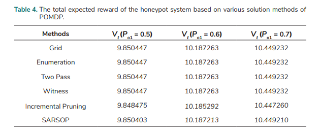
Analyses over an infinite planning horizon for a discounted POMDP of the honeypot system are performed. Let P_a = 0.6, P_d = 0.6, E_o = 1, E_r = 2.5, B_i = 16, E_l = 14, and γ = 0.85. The following solution methods or algorithms [23, 24, 26–29, 30] are used to solve the POMDP problem: Grid, Enumeration, Two Pass, Witness, Incremental Pruning, and SARSOP. The total expected reward of the honeypot system based on POMDP is denoted by V_t in this paper. The values of V_t at three different observation probabilities of receiving commands (P_o1 = 0.5, 0.6, and 0.7) are computed using various solution methods of POMDP. The result of V_t is shown in Tab. 4. The values of Incremental Pruning and SARSOP are very close to the results of the other four methods and the results of the four methods are the same.

Table 4. The total expected reward of the honeypot system based on various solution methods of POMDP.

5.3. The Analysis for the Honeypot System with Various Observation Probabilities of Receiving Commands

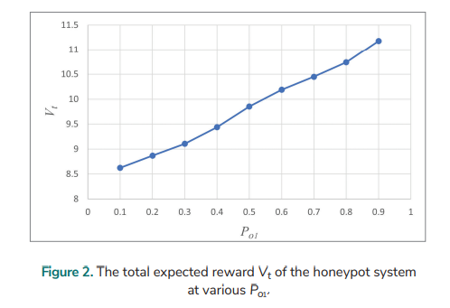
The total expected reward V_t of the honeypot system with various observation probabilities of receiving commands (P_o1) is analysed for the discounted POMDP over an infinite planning horizon. Grid is used to solve the POMDP problem. It tries to approximate the value function over an entire state space according to the estimation for a finite number of belief states on the chosen grid [31]. The following data are used in the analysis: P_a = 0.6, P_d = 0.6, E_o = 1, E_r = 2.5, B_i = 16, E_l = 14, and γ = 0.85; P_o1 = 0.1, 0.2, 0.3, …, 0.9. Fig. 2. shows that the total expected reward V_t of the honeypot system increases as the observation probability (P_o1) of receiving commands rises. In the following sections of this paper, the Grid method is also used in solving the POMDP problem.

Figure 2. The total expected reward Vt of the honeypot system at various Po1

5.4. Analyses for the system with various Pa and Pd

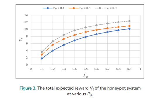
An analysis for the discounted POMDP with various P_a over an infinite planning horizon is conducted. The following data are utilised: P_d =0.6, E_o = 1, E_r = 2.5, B_i = 16, E_l = 14, and γ = 0.85. The total expected reward V_t of the honeypot system at various P_a for various P_o1 is analysed and the result is shown in Fig. 3. V_t increases with higher values of P_a, although the rate of increase steadily diminishes. The increased P_a provides the honeypot with more opportunities for collecting valuable information about attackers. V_t is larger when P_o1 is larger.

Figure 3. The total expected reward Vt of the honeypot system at various Pa

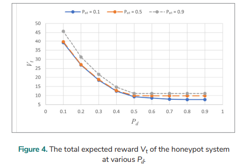
Let P_a = 0.6, E_o = 1, E_r = 2.5, B_i = 16, E_l = 14, and γ = 0.85. The V_t at various P_d for various P_o1 is analysed over an infinite planning horizon, and Fig. 4. shows the results. V_t is higher when P_o1 is higher, but the value of V_t when P_o1 = 0.1 is very close to that of V_t when P_o1 = 0.5 (if P_d < 0.5). For P_o1 = 0.1, V_t falls as P_d is increased from 0.1 to 0.8 and is unchanged when P_d moves from 0.8 to 0.9; for P_o1= 0.5, V_t decreases as P_d is increased from 0.1 to 0.6 and is unchanged as P_d goes from 0.6 to 0.9; for P_o1 = 0.9, V_t declines as P_d is increased from 0.1 to 0.5, though it does not change as P_d moves from 0.5 to 0.9. There is no significant difference in V_t for P_o1 = 0.5 and P_o1 = 0.9 when P_d changes from 0.5 to 0.9.

Figure 4. The total expected reward Vt of the honeypot system at various Pd

5.5. Analyses for the System with Various Transition Rewards

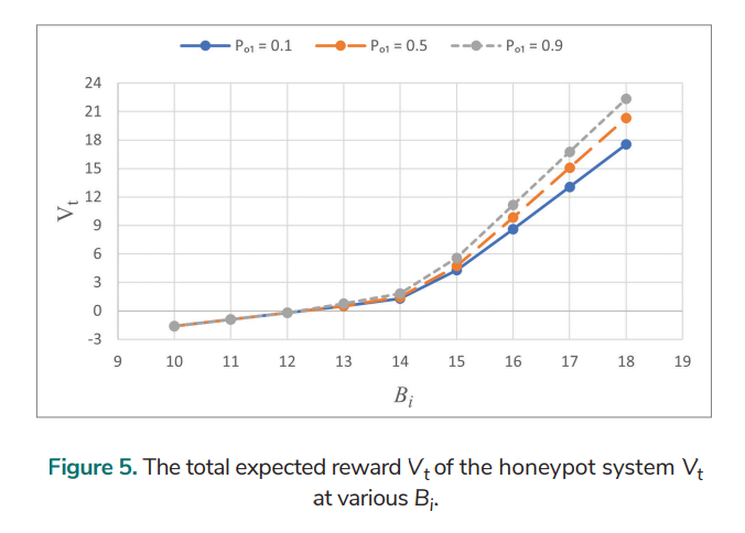
Analyses for the honeypot system with various transition rewards over an infinite planning horizon are performed. The following data are utilised: P_a = 0.6, P_d = 0.6, E_o = 1, E_r = 2.5, E_l = 14, and γ = 0.85. The total expected reward V_t at various P_a for various P_o1 is analysed, and the results are shown in Fig. 5. V_t initially increases slightly (B_i < 14) and then more rapidly (B_i > 14) with the increase of B_i . V_t for various P_o1(0.1, 0.5, and 0.9) is the same when B_i = 10, 11, and 12. V_t is the same for P_o1 = 0.1 and 0.5 when B_i = 13. When B_i > 13, V_t is larger if P_o1 is larger.

Figure 5. The total expected reward Vt of the honeypot system Vt at various Bi .

Figure 6. The total expected reward Vt of the honeypot system at various El .

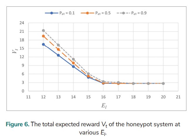
Let P_a = 0.6, P_d = 0.6, E_o = 1, E_r = 2.5, B_i = 16, and γ = 0.85. The total expected reward V_t at various E_l for various P_o1 is analysed over an infinite planning horizon and Fig. 6. shows the results. V_t decreases when E_l is increased from 12 to 16. V_t is the same for P_o1 = 0.1 and 0.5 as E_l rises from 17 to 20. It is the same for all the three values of P_o1 (0.1, 0.5, and 0.9) when E_l goes from 19 to 20.

The MDP-based predictive modelling for the honeypot system has demonstrated that the model and algorithms in this paper are suitable for performing analyses over both a finite planning horizon and an infinite planning horizon (for a discounted MDP), and that they are effective at finding an optimal policy and maximizing the total expected rewards of the states of the honeypot system. The results of the total expected reward using Gauss-Seidel’s algorithm of VI, PI, and LP are the same, and the result of Q-learning is very close to the same result, indicating the MDP model created in this paper is valid and that the model parameters are suitable.

In the predictive modelling of the honeypot system based on the discounted POMDP over an infinite planning horizon, the total expected reward V_t of the honeypot system increases with the increase of the observation probability of receiving commands (P_o1). It also rises as P_a is increased or B_i is increased. The increased P_a leads to more opportunities for the honeypot to collect valuable information about attackers. As P_d increases, V_t declines at first and then levels out. As E_l increases, V_t decreases by successively smaller amounts until it eventually flattens out.

The authors in this paper do not have any competing interest.

No database or dataset was used or generated in the research of this article.

This paper is based upon work supported by Mississippi State University (MSU) in the USA.